This project allowed me to learn how to implement ray tracing and render images with different lighting constraints. First, I implemented the methods for ray tracing through pixels including different intersection algorithms depending on the primitive type (triangle, versus sphere). Then, I created a binary tree structure for a Bounding Volume Hierarchy in order to accelerate rendering and calculation of ray intersections, using bounding boxes instead. Afterwards was the fun part, implementing different illumination rendering sample techniques, and experimenting with different sampling, ray depth, and light ray parameters. Lastly, implemented adaptive sampling to even better accommodate large sample sizes and efficiently sample.
Part 1: Ray Generation and Intersection
This portion of the project set up a lot of the basics for the rest of Pathtracer. After using gridSampler->get_sample() to gather ns_aa random samples through the input pixel, we needed to generate a ray for each of them. Generating rays required taking the normalized x and y positions passed in as input and converting them to the camera space first. This involved some calculations on both the x and y components; after transforming from image space to camera space, I was able to create a Ray object with the camera position as the origin, and the camera-to-world matrix multiplied by the camera space-transformed coordinate as the direction. Lastly, setting the min and max times to the nClip and fClip values so that we are not considering any parts of rays outside of the camera’s immediate field of view. For intersecting primitives, I followed the lecture slides for Moller-Trumbore Algorithm (for Triangles), and sphere intersection.
For the triangle intersection, I implemented the Moller-Trumbore algorithm, as mentioned above. This takes advantage of barycentric coordinates to rewrite the ray-intersection equation o + td into barycentric coordinate form. From there, the algorithm is deduced using matrix form, cramer’s rule and the determinants. The outputs are the barycentric coordinates and the time t of intersection. Moller-Trumbore will also always give the nearest intersection. Using these results I checked if the ray intersection occurred, and then filled in the required parameters of the Intersection objects.
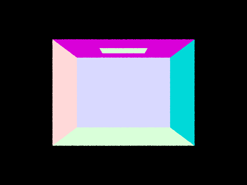 CBempty.dae
|
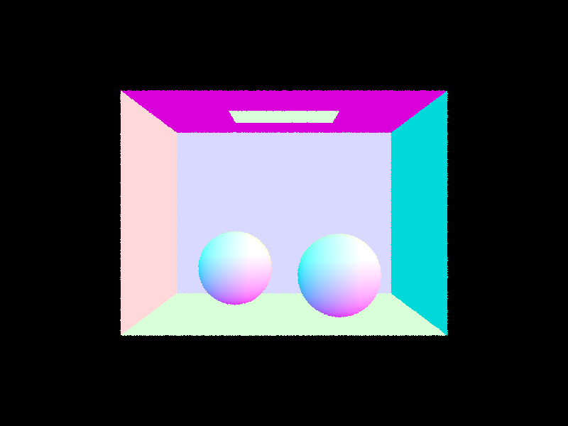 CBspheres.dae
|
Part 2: Bounding Volume Hierarchy
The BVH construction required implementing a binary tree. After iterating through all primitives and adding them to a bounding box, then creating a BVHNode with that bounding box, I check if it’s < max_leaf_size. If yes, set the required node parameters and return. Otherwise, I needed to recursively split the primitives into left and right children nodes until those respectively all had < max_leaf_size primitives themselves. The heuristic I chose was relatively simple - I first chose the axis with the longest range, and split on that axis at the centroid point. I added an additional clause where if all the primitives ended up on one side of the heuristic, I removed the last primitive from the full child node and added that to the empty one instead.
When not using the BVH algorithm, cow.png took around 40 seconds - 1 minute to render on my laptop, and I had to stop my program after over 2-3 minutes for both CBlucy and maxplanck because the rendering was taking a very long time. However, once BVH was implemented, all three of these files rendered within 1 second on 8 threads using my laptop, which is extremely fast!
The issues that I ran into while implementing this section were relatively minor (thankfully!), such as miswriting max for min while checking my bbox bounds, or other typos of the like.
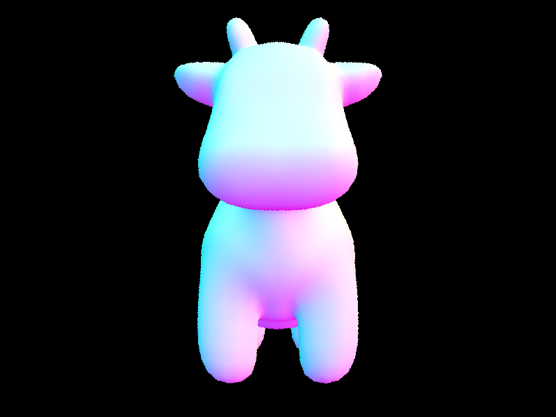 cow.dae
|
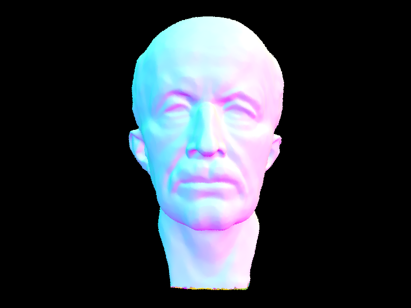 maxplanck.dae
|
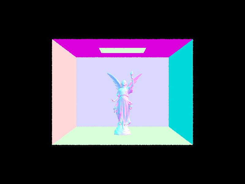 CBlucy.dae
|
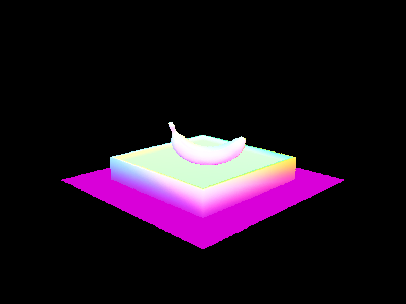 banana.dae
|
Part 3: Direct Illumination
For direct lighting implementation, there were two types: via uniform hemisphere sampling, and via importance sampling using the lights. Uniform hemisphere sampling implementation provided the framework for importance sampling. To implement, I sampled from a uniform hemisphere sampler num_samples times, using the Intersection bdsf passed into the function. Once my incident angle and its corresponding pdf are populated, then I can convert the incident direction to world space to create a ray from the hit point in the direction of the incident ray, offset by EPS_D to mitigate precision issues. If this ray intersects with a light source, then I compute the irradiance by using the mathematical equations in lecture slides and accumulate it to the Monte Carlo estimation, making sure to normalize by the sample’s pdf and the total number of samples.
From there, importance sampling implementation followed - instead of iterating through num_samples, I iterated through all lights in the scene, as importance sampling samples lights directly for smarter sampling. If the light is a delta light, then we only need to take one sample, since all the samples would be the same. Otherwise, for each non-delta light we sample ns_area_light times. Since sampling from lights populates the incoming radiance in world space, I can use that for all ray and intersection calculations, and converting to object space retrieving the Spectrum and calculating the Monte Carlo estimation. Once I had all my variables, I checked if the incoming radiance was in front of the light (the z coordinate is greater than 0), and if that was the case, then I cast a shadow ray from the hit point to the light source to check for intersections with other primitives within the scene. If there was no intersection, then calculations for Monte Carlo estimation followed as in the hemisphere sampling, normalizing by the sampled pdf, and ns_area_light if the light was not a delta light (1 if delta light).
Issues that I ran into included making sure that I was taking the sampled radiance’s intersection emission, and not the input intersection’s emission twice. Additionally, I realized that I had a bug in my bounding box intersection, where my constraints were too tight and I was not considering rays that originate within the bounding box itself as an intersection (when they should be!). Lastly, the killer bug was realizing that C++ parses a < b < c as (a < b) < c, and is nowhere near equivalent to (a < b) and (b < c) which I had in my triangle intersection. After fixing that, everything ran perfectly. Amazing.
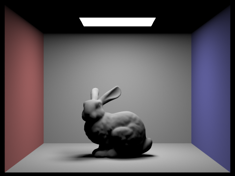
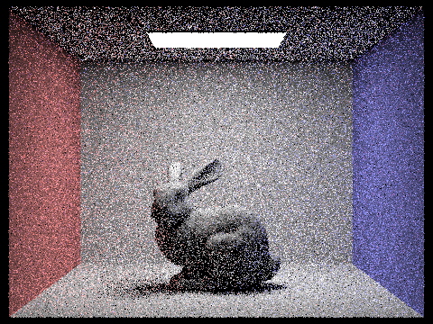
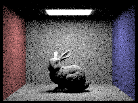 CBbunny.dae with Uniform Hemisphere Sampling
|
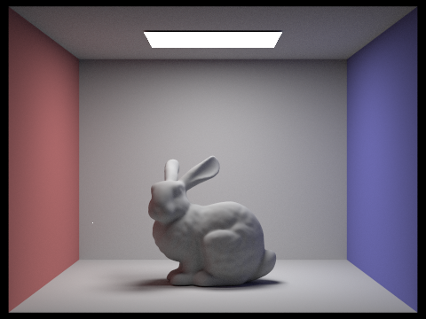
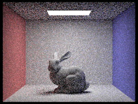
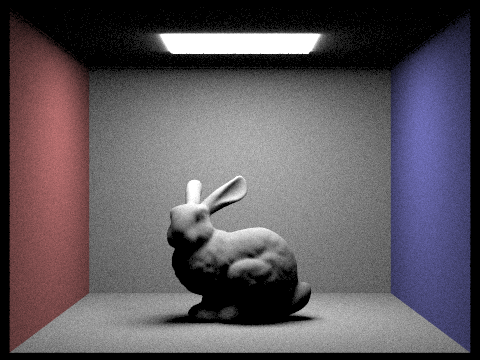 CBbunny.dae with Importance Sampling
|
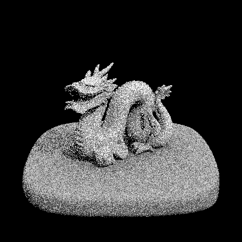
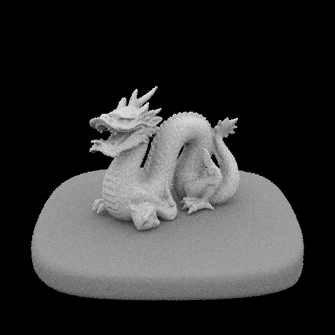
 dragon.dae with Importance Sampling
|
 dragon.dae with Importance Sampling s = 1, l = 1
|
 dragon.dae with Importance Sampling s = 1, l = 4
|
 dragon.dae with Importance Sampling s = 1, l = 16
|
 dragon.dae with Importance Sampling s = 1, l = 64
|
In terms of the differences between Uniform Hemisphere and Importance Sampling: Computationally, the difference of importance sampling was marginally better, and due to my implementation neither method stood out. However, the difference to the naked eye is staggering - uniform hemisphere sampling rendering is much noisier and less clear than those from importance sampling. Since importance sampling prioritizes samples which will actually contribute to the rendering, there is more input from samples which will produce non-zero radiance, resulting in a clearer, smoother image.
Part 4: Global Illumination
Indirect lighting uses Russian Roulette as an unbiased way of deciding sampling termination, in order to lessen the amount of computation that would be required to render a scene. Implementing indirect lighting was rather straightforward, following pseudocode from lecture slides. First, I accumulate a one bounce radiance to get started, as this sets the scene for all of the bounces following, which are the indirect radiances. To accomplish ray depth cutoff, I checked if the current input ray’s depth was greater than 1, then there must be at least one bounce that can be calculated, and so if that case and the Russian Roulette cpdf probability (I used 0.6) both returned true, then I would sample an incoming irradiance from the current intersection, and create a new Ray going from the current hit point in the direction of the world-space incoming radiance, decrementing the depth of this new ray by 1. If this new ray intersected with my BVH of the scene, then we know that it is refracted on a different point and we can recursively add to the Monte Carlo estimation with another call to at_least_one_bounce_radiance, normalizing by both the pdf and the Russian Roulette probability.
A tricky part that I had while debugging due to my unfamiliarity with C++ was having unnecessary Intersection elements created, and trying to pass those pointers into the intersect functions, when I should have simply been passing in an address and thus reusing the memory. After fixing my memory leak issues, my renders ran perfectly on the Hive machines instead of being killed off.
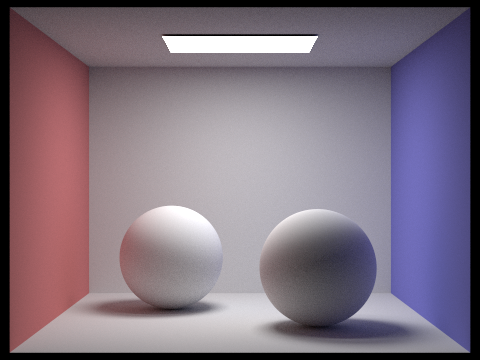 CBspheres_lambertian.dae with Global Illumination s = 1024
|
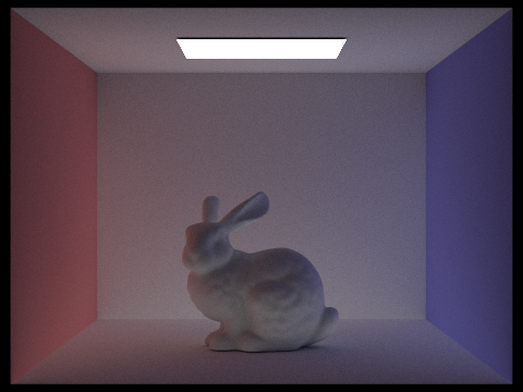
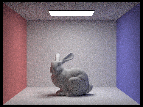
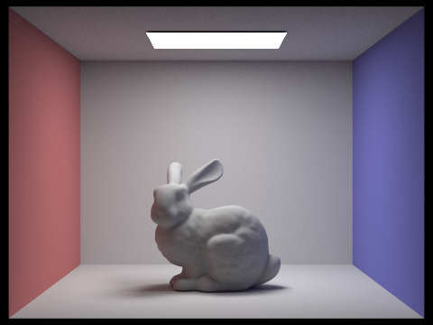 CBbunny.dae with Global Illumination s = 1024
|
 CBbunny.dae with Direct Illumination s = 1024
|
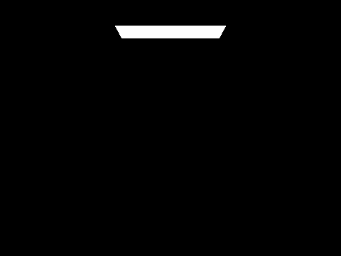
 CBbunny.dae with Indirect Illumination s = 1024
|
 CBbunny.dae s = 1024 m = 0
|
CBbunny.dae s = 1024 m = 1
|
 CBbunny.dae s = 1024 m = 2
|
|
CBbunny.dae s = 1024 m = 3
|
 CBbunny.dae s = 1024 m = 100
|
 CBbunny.dae s = 1 l = 4
|
 CBbunny.dae s = 2 l = 4
|
 CBbunny.dae s = 4 l = 4
|
 CBbunny.dae s = 8 l = 4
|
 CBbunny.dae s = 16 l = 4
|
 CBbunny.dae s = 64 l = 4
|
 CBbunny.dae s = 1024 l = 4
|
Part 5: Adaptive Sampling
For adaptive sampling, I followed the algorithm given in the spec, adding a check where if the iteration % 32 that I was currently on was 0, then I would perform the calculations to check if the rays had converged. If they had, then I went ahead and updated my sampleCountBuffer and sampleBuffers, and broke out of the for loop. This meant that the rays would stop tracing through that pixel, and could move onto the next pixel, therefore lessening computation where possible.
 CBbunny.dae with Adaptive Sampling l = 1 m = 5
|
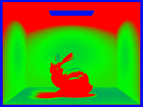 Sampling Rate png of CBbunny.dae with Adaptive Sampling l = 1 m = 5
|